
Will It Make Any Difference? How Our Receive Antennas Evolved
Will It Make Any Difference? How Our Receive Antennas Evolved
A broken loop started the project. Keeping useful signals alive through the antenna, feedline and receiver became the reason to keep improving it.
RF.Guru-werkdefinitie: Common-modestroom is de niet-opgeheven fasorsom van de stromen in een gespecificeerde geleiderset, beoordeeld in een gedefinieerde doorsnede en met een verklaarde conventie voor de stroomrichting. In de bedoelde differentiële transmissielijnmodus zijn de heen- en retourstromen gelijk en tegengesteld, zodat hun fasorsom nul is. Wanneer ze elkaar niet opheffen, moet de resterende stroom zich sluiten via een ander referentie- of retourpad—zoals de buitenzijde van een coaxafscherming, een mast, een apparatuurchassis, stationsbekabeling, nabije structuren, aarde, de operator of gedistribueerde koppeling via de omgeving.
Deze bredere werkdefinitie is bijzonder bruikbaar in praktische antennesystemen. Bij zenden kan niet-opgeheven stroom op de buitenzijde van de coax de voedingslijn en verbonden structuren deel maken van het stralende antennesysteem, tenzij dat pad bewust is gekozen, duidelijk is gedefinieerd en correct wordt beheerst—bijvoorbeeld met het vereiste retourpad en een geschikte common-mode-choke op de juiste grens.
Lees dit artikel in het Nederlands →
My trusted Wellbrook receive loop died. I still respect the electronics and the thinking behind it; the failure of my antenna was mechanical. For equipment that lives outdoors, that is not a side issue. It started a question that became years of work: could we build a receive antenna that was not merely different, but better as a complete system?
The Broken Loop That Started the Project
My son Jonas began designing the mechanical parts. I started on the electronics. The ambition was quite direct: beat the Wellbrook. But “beat” needed a better definition than making the S-meter climb.
I wanted connectors, supports, strain relief and weather protection that would keep doing their job outdoors. Electrically, I wanted the wanted signal to survive local noise and strong unwanted signals without the installation becoming an uncontrolled part of the receiver. Jonas's mechanical work and my electronics were two parts of the same problem.
The first OctaLoop worked, and early adopters sent encouraging feedback. That was a beginning, not an answer to every question. Once two receive antennas are already doing a good job, another question becomes much harder: is the next change actually useful, or have I just caught a better band opening? That question stayed with me through the first six years of development.
What I Wanted the Revisions to Change
A revision should solve something. More output gain is easy to notice; a better receiving system is not always louder. The useful changes often happen where the mechanics, element, amplifier and feedline meet.
Mechanics That Preserve the Electrical Behaviour
Sealing, strain relief, stable connections and repeatable geometry matter because an outdoor antenna is still the same electrical circuit after rain, wind and temperature changes. A support that shifts, a connector that corrodes or moisture around a sensitive input can change the load and unwanted coupling. That was the lesson of the failed loop: a good amplifier is not the whole product.
This is a positive reason to refine the mechanics even when the dry-workbench response barely moves. The aim is to keep that response and the intended balance in service—not to put a different enclosure around the same unresolved problem.
Symmetry That Stops Interference Becoming Signal
Common-mode rejection became a guiding principle. At a balanced input, interference coupled similarly to both sides can be rejected. Unequal impedances, stray capacitances or response paths can turn part of it into a differential signal, which the amplifier then treats like wanted information.
This is why an impressive amplifier specification cannot stand in for the complete antenna. The element, protection, connections, mechanics and nearby conductors influence what actually reaches the input. Analog Devices' difference-amplifier analysis illustrates the underlying point: imperfectly matched paths convert common-mode voltage into an output error.
Common-mode rejection ratio, or CMRR, compares differential gain with common-mode gain at a specified interface and frequency: CMRR = 20 log10(|Ad/Ac|). It does not describe rejection of every local noise source. Interference already arriving in the wanted differential mode, or as a wanted-looking field, is not removed by calling the amplifier balanced.
Headroom and Response, Not Just a Lower Noise Figure
Strong unwanted signals can drive a front end into compression or generate intermodulation products. Suitable filtering and more linear headroom can prevent those products from burying a weak station. If that is the limiting problem, fixing it is more useful than adding gain to both the wanted signal and the trouble.
Likewise, once receiver-added noise is comfortably below the noise delivered by the antenna, shaving another fraction from the amplifier's noise figure may have little effect on installed SNR. At a quieter site, on a different band or with a lower-output element, that balance can change. ITU-R P.372 separates atmospheric, galactic and man-made radio noise precisely because one universal noise-floor assumption is not enough.
Some development changes refine layout, matching or mechanics. Others reconsider the circuit topology itself; TerraBooster was one such branch of our development story. A topology change opens different choices for transfer response and headroom. It is a different engineering job from adjusting a component value, not a promise that every redesign must deliver a dramatic SNR increase.
Why the Far Field Was Not the Whole Answer
We used far-field testing. It remains valuable for response, pattern, nulls and sensitivity under a defined electromagnetic stimulus. It answers important antenna questions; it is not made obsolete by a focus on common-mode rejection.
But a clean test signal does not recreate every unwanted path in a working station. Interference can arrive along coax, through a mast or power lead, or through unequal coupling to nearby objects. I wanted to know how the whole installation behaved as well as how the antenna responded to the wanted field.
That meant connecting bench and field results. Balance tests address common-mode conversion; strong-signal tests address overload; calibrated sweeps address response; outdoor records address mechanical consistency. The long-term reception comparison asks whether the relevant benefit survives all the way to the receiver.
The Question Took Me to Lombardsijde—and a Database
I left the comparison problem alone for a while, but it kept returning. Eventually I built the database behind spots.rf.guru. I wanted more than a favourite screenshot: reception records over days and weeks, through quiet periods, noisy periods and changing propagation.
Lombardsijde is not an idyllic interference-free test range. Our urban receiving site has LED floodlight interference and limits on mast height. That makes the complete-system question very real. A mechanically tidy loop and a low-noise first stage still have to coexist with the site and its feedlines.
People email asking why New Zealand, Australia and Japan appear in the logs. My answer starts with propagation: when the path is open, it is open. Our task is to avoid losing the available signal-to-noise ratio locally. Common-mode control, sensible filtering and headroom are ways to do that; none manufactures an ionospheric opening.
The Advantage Should Follow the Antenna
Our long-run comparison approach has been to operate two candidates together at the same site, about six metres apart, for a month, then exchange their positions and continue. They see the same broad openings and transmitting activity. The position swap asks whether the apparent advantage belongs to the design or to a better patch of ground.
Six metres is a practical spacing, not proof of isolation or identical noise. The antennas can still couple, and a fence, cable route or local interference source can favour one location. If the better result remains at that location after the swap, it is not yet an antenna advantage. The same logic applies to an unequal receiver channel.
| Part of the comparison | Question it answers |
|---|---|
| Simultaneous reception | Did both antennas experience the same transmission and broad propagation interval? |
| Physical position swap | Does the effect follow the antenna rather than the location? |
| Independent cable/channel swap | Does a receiver, feedline or bias path explain the apparent difference? |
| Repeated operating blocks | Does the result recur across the intended bands and relevant noise conditions? |
A rapid switch into one receiver is another useful method when switching is fast compared with fading. Its loss, isolation, settling and unused-port termination become part of the test. With two simultaneous receivers, channel calibration, filtering, clocking and overload state need the same attention. An A/B label by itself does not remove those differences.
Do Not Let the Test Flatter the New Design
Before a comparison, define what would count as useful: wanted-signal transfer, installed SNR, decode reliability or mechanical consistency. Record height, orientation, cables and common-mode boundaries, then keep receiver gain, filtering, bandwidth, decoder software and reporting rules consistent. A changed gain setting can look surprisingly like progress.
Compare the same transmissions in matched time windows. Record wanted signal and noise separately where possible: an SNR improvement can come from more wanted signal, less coupled noise or both. Keep A-only and B-only decodes too. Looking only at transmissions both antennas decoded throws away exactly the marginal cases that may matter most; synchronized recordings or an independent transmission record are needed to identify intervals neither decoded.
Thousands of spots from the same opening are not thousands of independent experiments. Look for repeatability across separate sessions, bands and noise conditions, not only the most flattering total. Calibration limits and the spread between those blocks belong alongside the estimated difference. The NIST uncertainty framework is useful here: uncertainty explains how well a result is known, not why nothing can be known.
The Maps Show the Station at Work
The maps below come from reported decodes archived for the Lombardsijde receiving systems. They show real reception activity, not a simulated radiation pattern or a controlled revision-versus-revision result. The plates refresh at their existing URLs; their reporting window and displayed totals belong to the image being viewed.
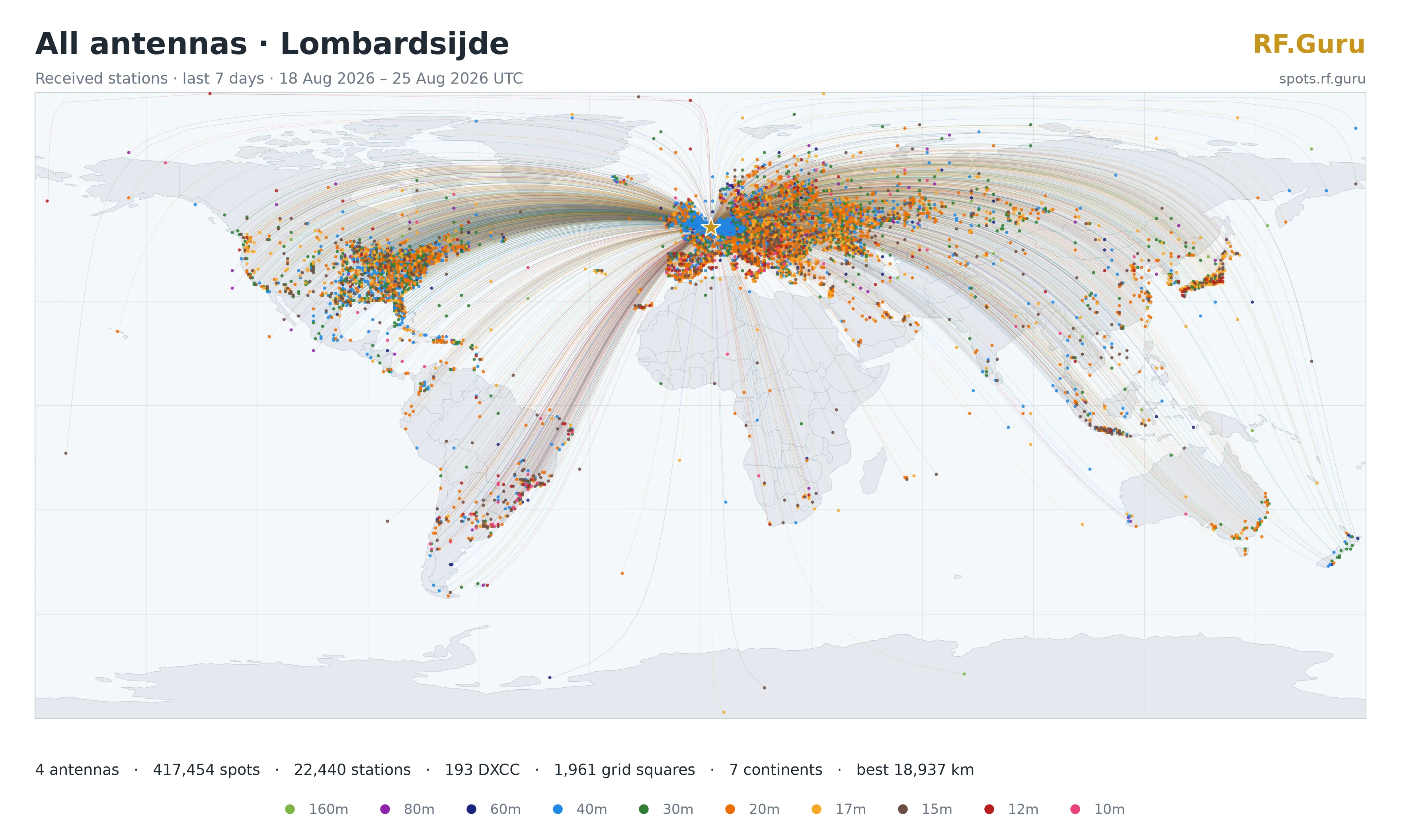
Read the Filters as Numbers, Not as Operating Modes
The PSKReporter developer specification makes clear that data gathering depends on the reporting client. It carries fields for SNR, mode and decoder software. The WSJT-X guide uses a 2500 Hz reference noise bandwidth for its signal reports; that convention must not silently be assigned to every reporting client.
The two filtered plates retain submitted SNR values at or above −18 dB and 0 dB. The filenames retain their historical “cw” and “ssb” shorthand, but those labels do not convert digital decodes into human readability. Receiver bandwidth, interference, fading, mode and operator skill still matter. If every stored report exceeds a selected threshold, a filtered map can legitimately look identical to the unfiltered one.
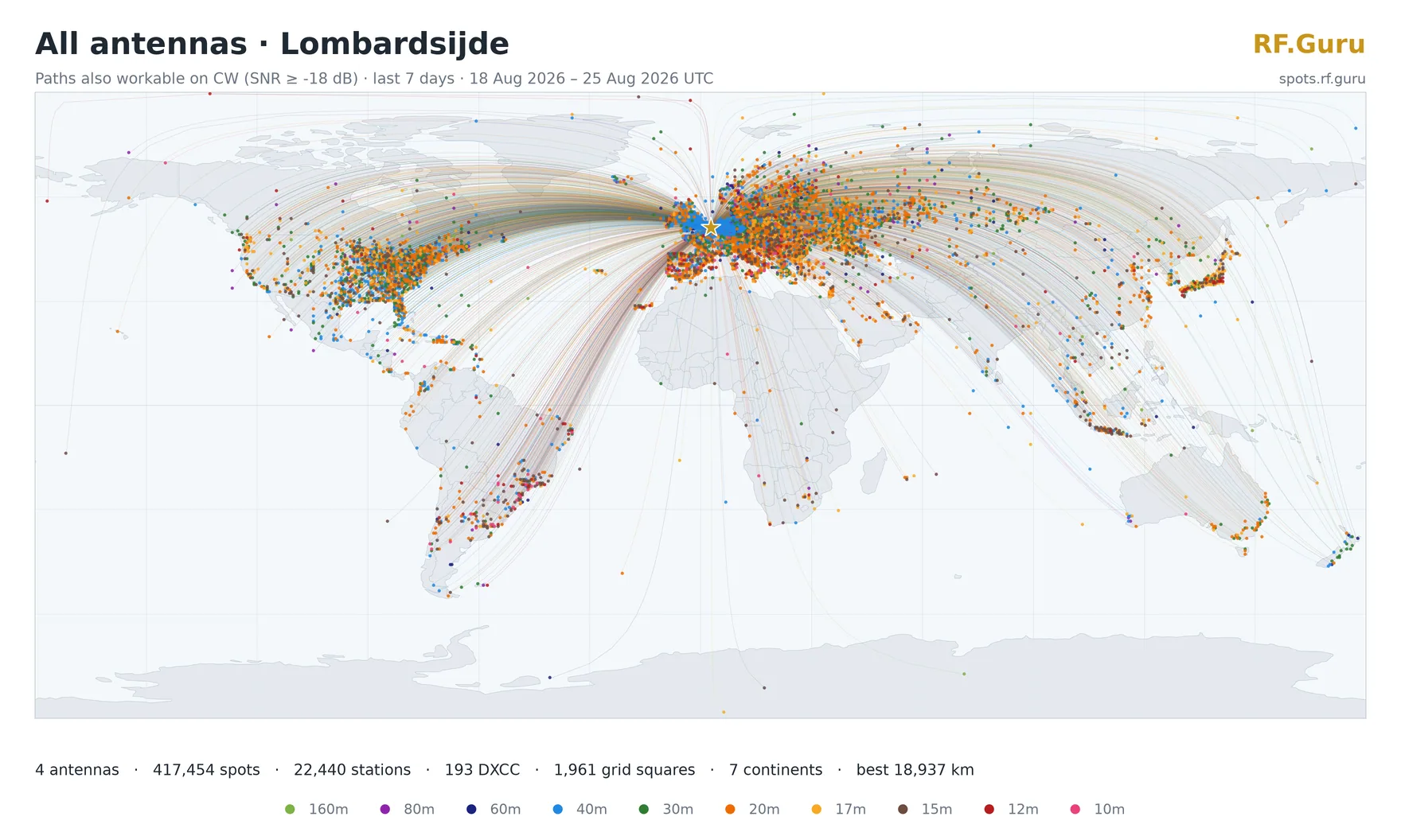
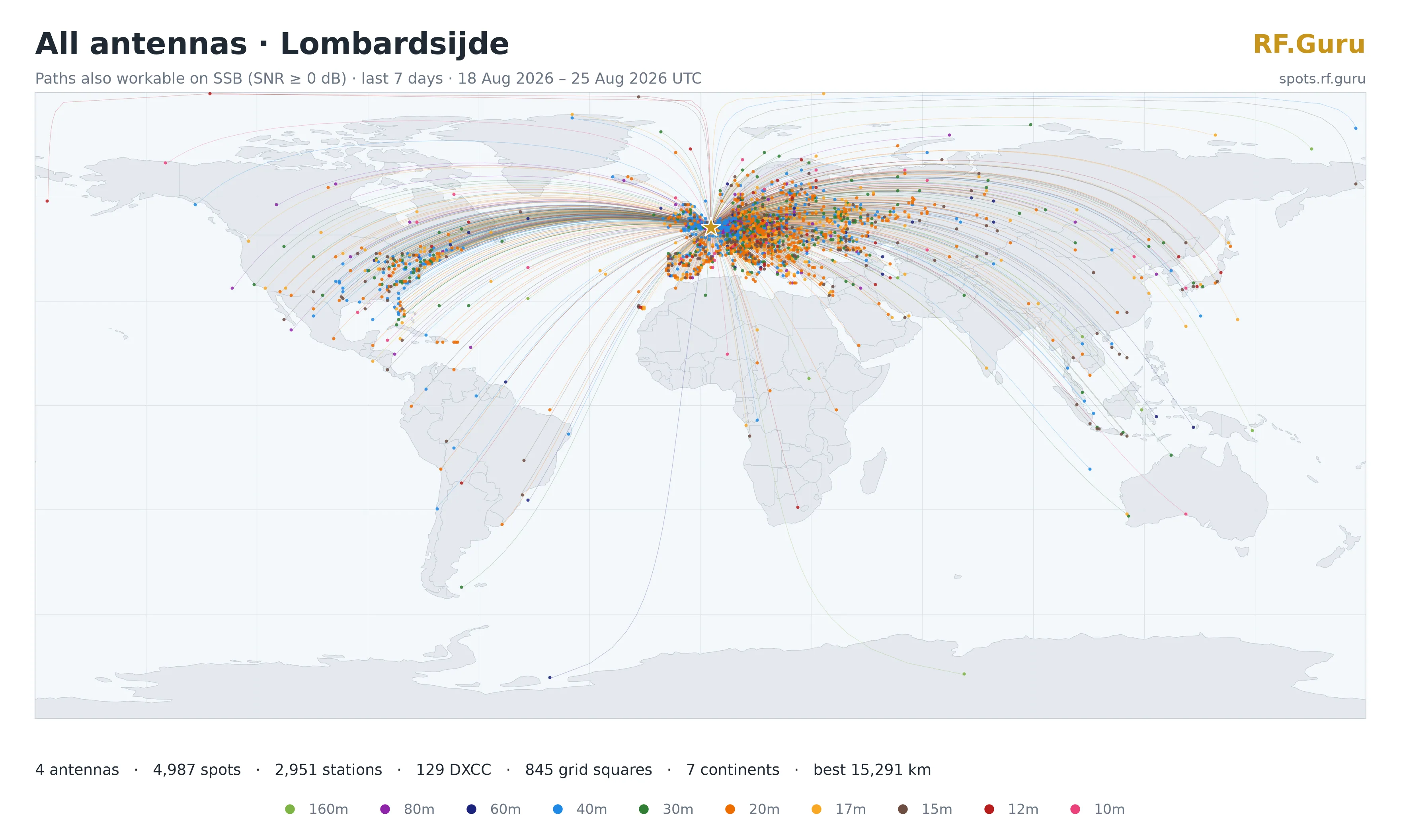
You can explore the archive at spots.rf.guru and listen through sdr.rf.guru. Those views show what the station is hearing. A numerical revision comparison still needs its paired records, receiver settings and calibration; a busy world map cannot supply those on its own.
So, Will It Make Any Difference?
Yes—a revision can make a worthwhile difference without making an antenna sound like a different class of product. Near a decode or copy threshold, a modest repeatable SNR improvement can turn an unsuccessful reception into a successful one. Away from that threshold, the same change may be hard to notice. Better sealing or more stable mechanics may show their value over seasons rather than in a quick listening test.
That is why I keep refining the designs. I want the mechanics to preserve the electrical behaviour, the input to avoid converting local interference into signal, and the front end to remain useful when strong signals arrive. The comparison work exists to distinguish those benefits from a lucky location or a good afternoon on the bands.
It also explains why “newer” is not a sufficient reason to replace an antenna that already serves you well. Start with the limitation you want to solve. An improvement in overload behaviour matters when overload is the problem; better common-mode control matters when that unwanted path is significant.
From the failed Wellbrook to the later revisions, the ambition stayed the same: build a complete receiving system that keeps doing its job outdoors and gives the available signal a better chance to survive the local environment. That is a more useful difference than a bigger number on the S-meter.
Mini-FAQ
- What started RF.Guru's receive-loop project? My own Wellbrook loop suffered a mechanical failure. Jonas began developing the mechanics while I worked on the electronics, aiming for a complete receive system that would perform consistently outdoors.
- What can improve without a louder S-meter reading? Better balance and common-mode control can reduce coupled interference; more linear headroom can reduce overload products; sealing and stable mechanics can preserve behaviour over time. The useful result depends on the installation.
- Does high CMRR reject every local noise source? No. It rejects the common-mode component at the specified interface. Interference already converted to differential mode, or arriving like the wanted field, is not removed simply by a high amplifier CMRR.
- Why swap antenna positions and receiver channels? Position swaps expose site bias, while separate cable or channel swaps expose signal-chain bias. A candidate-specific advantage should follow the antenna rather than a favourable location or receiver.
- Are the filtered maps CW or SSB reception tests? No. They retain submitted digital reports at or above −18 dB or 0 dB. Those numerical filters do not predict human copy or turn digital reports into CW or SSB contacts.
- Can a small improvement matter? Yes. Near a detection or copy threshold, a modest repeatable SNR improvement can change an outcome. It need not look dramatic on an S-meter, and it does not guarantee an extra decode on every transmission.
- Must I replace an antenna that already works well? No. Start with the limitation you want to solve: noise coupling, overload, a response gap or outdoor reliability. A revision is useful when it addresses that limitation, not merely because its label is newer.